Fourier Transform

Recap

• What is a complex number?
• What is the trigonometric form of a complex number?
• What is the difference between the cartesian and polar coordinate system?

• How to compute $r$ and $\varphi$ using $\Re$ and $\Im$ and vice versa?

Conversion

Polar $\rightarrow$ cartesian

\begin{equation} \Re=A \cos \varphi \\ \Im=A \sin \varphi \\ \end{equation}

Cartesian $\rightarrow$ polar

\begin{equation} A = \sqrt{\Re^2+\Im^2} \\ \varphi = \text{atan2}(\Im,\Re) \approx \arctan \left(\frac{\Im}{\Re}\right) \end{equation}

Euler formula

\begin{equation} z=\Re + i\cdot\Im \\ z=A\cdot(\cos{\varphi} + i\cdot\sin{\varphi})\\ e^{ix}=\cos{x}+i\sin{x} \\ z=A\cdot e^{i\varphi} \end{equation}

Taylor series

\begin{equation} f(x) = f(a) + \frac{f'(a)}{1!} (x-a) + \frac{f''(a)}{2!} (x-a)^2 + \frac{f'''(a)}{3!} (x-a)^3 +\ldots \end{equation}\begin{equation} f(x) = \sum_{n=0}^{\infty} \frac{f^{(n)}(a)}{n!} (x-a)^n \end{equation}

• where $f^{(0)}(x)=f(x)$ and $0!=1$
• for $a=0$ also known as Maclaurin series

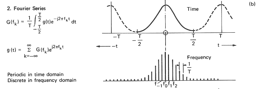
Fourier series

• for orthogonal functions $g_1\ldots g_n$ and coefficients $a_1\ldots a_n$ let us define:

\begin{equation} f(t)=a_1\cdot g_1(t) + a_2\cdot g_2(t) + a_3\cdot g_3(t) + \ldots + a_n\cdot g_n(t) = \sum_{n=1}^{\infty}a_n\cdot g_n(t) \end{equation}

• let us take $g_1$ use it to multiply both sides of the above equation:

\begin{equation} g_1(t)\cdot f(t)=a_1\cdot g_1^2(t) + \sum_{n=2}^{\infty} a_n\cdot g_n(t)\cdot g_1(t) \end{equation}

• let us also compute the integral of both sides of the equation:

\begin{equation} \int_{t_1}^{t_2} g_1(t)\cdot f(t) dt=\int_{t_1}^{t_2} a_1\cdot g_1^2(t)\ dt + \sum_{n=2}^{\infty} \int_{t_1}^{t_2} a_n\cdot g_n(t)\cdot g_1(t)\ dt \end{equation}

Fourier series

• because all the components are orthogonal their products are always 0,
  • we can therefore remove most of the equation:

\begin{equation} \int_{t_1}^{t_2} g_1(t)\cdot f(t)\ dt=\int_{t_1}^{t_2} a_1\cdot g_1^2(t)\ dt = a_1\cdot \int_{t_1}^{t_2} g_1^2(t)\ dt \end{equation}

• to compute the coefficient $a_1$ we can simply use:

\begin{equation} a_1=\frac{\int_{t_1}^{t_2} g_1(t)\cdot f(t)\ dt}{\int_{t_1}^{t_2} g_1^2(t)\ dt} \end{equation}

• we can use a similar equation for all other coefficients:

\begin{equation} a_n=\frac{\int_{t_1}^{t_2} g_n(t)\cdot f(t)\,dt}{\int_{t_1}^{t_2} g_n^2(t)\ dt} \end{equation}

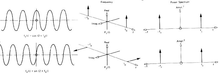
Trigonometric Fourier series

• Fourier used $\sin$ as the $g_n$ function:

\begin{equation} f(t) = \frac{A_0}{2} + \sum_{n=1}^{\infty}A_n\cdot\sin(n\omega_0t+\varphi_n) \end{equation}

(where $\omega_0=\frac{2\pi}{T_0}=2\pi f_0$ - ie. angular frequency, with unit rad/s)

• We can use the following equations:

\begin{equation} \sin(n\omega_0t+\varphi_n) = \sin(\varphi_n)\cos(n\omega_0t)+\cos(\varphi_n)\sin(n\omega_0t) \\ a_n=A_n\sin(\phi_n)\ \text{(by formula for $\Re$)} \\ b_n=A_n\cos(\phi_n)\ \text{(by formula for $\Im$)} \end{equation}

• To simplify the computation like this:

\begin{equation} f(t) = \frac{A_0}{2} + \sum_{n=1}^{\infty}a_n\cdot\cos(n\omega_0t)+b_n\cdot\sin(n\omega_0t) \end{equation}

Trigonometric Fourier series

\begin{equation} f(t) = a_0 + \sum_{n=1}^{\infty}a_n\cdot\cos(n\omega_0t)+b_n\cdot\sin(n\omega_0t) \end{equation}

• where $a_n$ and $b_n$ are known as the Fourier coefficients:

\begin{equation} a_0 = \frac{1}{T_0}\int_{0}^{T_0}f(t)\ dt \\ a_n = \frac{2}{T_0}\int_{0}^{T_0}f(t)\cdot\cos(n\omega_0t)\ dt \\ b_n = \frac{2}{T_0}\int_{0}^{T_0}f(t)\cdot\sin(n\omega_0t)\ dt \\ \end{equation}

Complex Fourier series

• We use the complex version of the Fourier formula more often:

\begin{equation} f(t) = \sum_{n=-\infty}^{\infty}F_n\cdot e^{in\omega_0t} \end{equation}

• where $F_n$ is computed:

\begin{equation} F_n=\frac{1}{T_0}\int_{0}^{T_0}f(t)\cdot e^{-i n\omega_0t}\ dt \end{equation}

Properties

\begin{equation} a_n=2\Re[F_n] \quad b_n=-2\Im[F_n] \end{equation}\begin{equation} F_0=a_0 \end{equation}\begin{equation} F_{-n}=F_n^{*} \quad |F_n|=|F_{-n}| \quad \angle(F_n)=-\angle(F_{-n}) \end{equation}

(Hermitian symmetry)

\begin{equation} a_n=(F_n+F_{-n}) \quad b_n=i\cdot(F_n-F_{-n}) \end{equation}\begin{equation} F_n=0.5\cdot(a_n-i\cdot b_n) \quad F_{-n}=0.5\cdot(a_n+i\cdot b_n) \end{equation}\begin{equation} A_n=\sqrt{a_n^2+b_n^2}=2|F_n| \end{equation}

Examples online

https://www.intmath.com/fourier-series/fourier-graph-applet.php

http://www.mathstools.com/section/main/fourier_series_calculator

Fourier transform

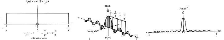
\begin{equation} F_n=\frac{1}{T_0}\int_{0}^{T_0}f(t)\cdot e^{-in\omega_0t}\ dt \end{equation}

• Fourier series is defined only for periodic signals (with the period $T_0$)!

• How can we compute the Fourier series for non-periodic signals?

  • Given that $\omega_0=\frac{2\pi}{T_0}=2\pi f_0$

  • If $T_0\rightarrow\infty$ then $\omega_0\rightarrow0$

  • Thus the $F_n$ coeffients will turn from a series of points $\rightarrow$ function of real values $F(\xi)$

\begin{equation} F(\xi) = \int_{-\infty}^{\infty} f(t)e^{-i 2\pi \xi t } dt \end{equation}

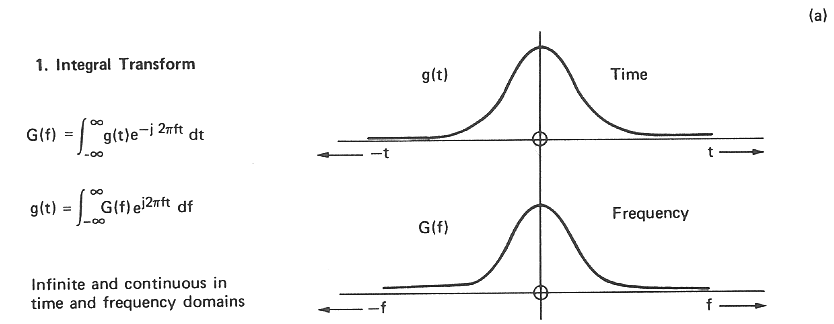
Fourier transform

• Analitic function

\begin{equation} F(\xi) = \int_{-\infty}^{\infty} f(t)e^{-i 2\pi \xi t} dt \end{equation}

• Synthetic function (aka. invrerse):

\begin{equation} f(t) = \int_{-\infty}^{\infty} F(\xi)e^{i 2\pi t \xi} d\xi \end{equation}

• Apart from the decomposition in the frequency domain, other useful forumlas include:
  • Amplitude spectrum: $|F(\xi)|$
  • Phase spectrum: $\angle[F(\xi)]$
  • Power spectrum: $|F(\xi)|^2$

When is it computable?

• finite energy: $\int_{-\infty}^{\infty}\lvert x(t) \rvert^2dt<\infty$
• finite number of extrema
• finite number of discontinuities
• any periodic signal (including inifinite energy)

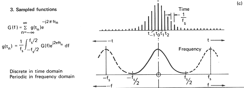
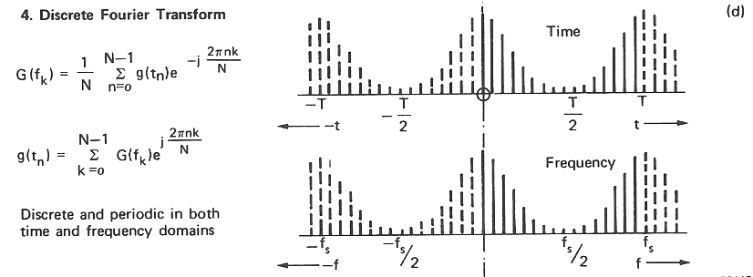
Discrete Fourier transform

• Used for digital signals

• Analitic function:

\begin{equation} X_k=\sum_{n=0}^{N-1} x_n e ^ {-i2\pi k n/N} \\ k \in 0\ldots N-1 \end{equation}

• Synthetic function (inverse):

\begin{equation} x_n=\frac{1}{N} \sum_{k=0}^{N-1} X_k e ^ {i2\pi k n/N}\\ n \in 0\ldots N-1 \end{equation}

Types of Fourier transforms

Fourier series

DTFT

DFT

Properties of the Fourier transform

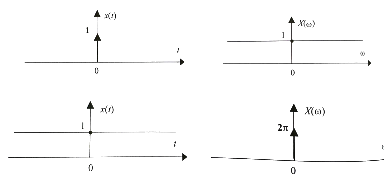
\begin{equation} f(t) \qquad\rightarrow\qquad F(\omega) \end{equation}

Inverse

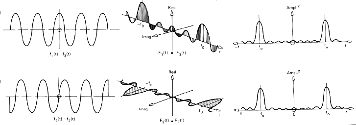
\begin{equation} F(t) \qquad\rightarrow\qquad 2\pi f(-\omega) \end{equation}

Convolution

\begin{equation} f_1\star f_2(t) \qquad\rightarrow\qquad F_1(\omega)F_2(\omega) \end{equation}

Product

\begin{equation} f_1(t)f_2(t) \qquad\rightarrow\qquad \frac{1}{2\pi}F_1\star F_2(\omega) \end{equation}

Shift

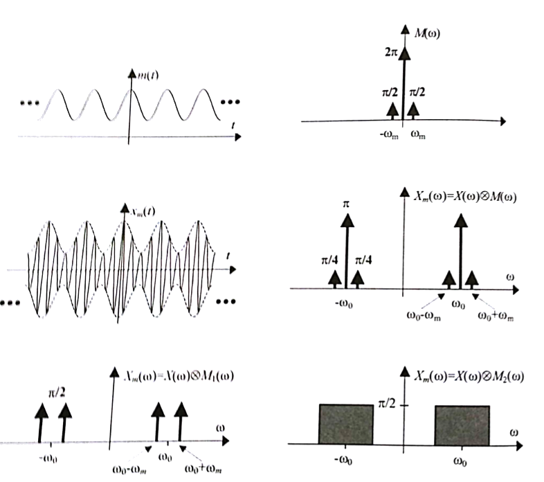
\begin{equation} f(t-u) \qquad\rightarrow\qquad e^{-iu\omega}F(\omega) \end{equation}

Amplitude modulation

\begin{equation} e^{i\xi t}f(t) \qquad\rightarrow\qquad F(\omega-\xi) \end{equation}

Scaling

\begin{equation} f(t/s) \qquad\rightarrow\qquad |s|F(s\omega) \end{equation}

Time derivative

\begin{equation} f^{(p)}(t) \qquad\rightarrow\qquad (i\omega)^{(p)}F(\omega) \end{equation}

Frequency derivative

\begin{equation} (-it)^{(p)}f(t) \qquad\rightarrow\qquad F^{(p)}(\omega) \end{equation}

Complex conjugation

\begin{equation} f^{\star}(t) \qquad\rightarrow\qquad F^{\star}(-\omega) \end{equation}

Hermitian symmetry

\begin{equation} f(t)\in \mathbb{R} \qquad\rightarrow\qquad F(-\omega)=F^{\star}(\omega) \end{equation}

A bit more on symmetry

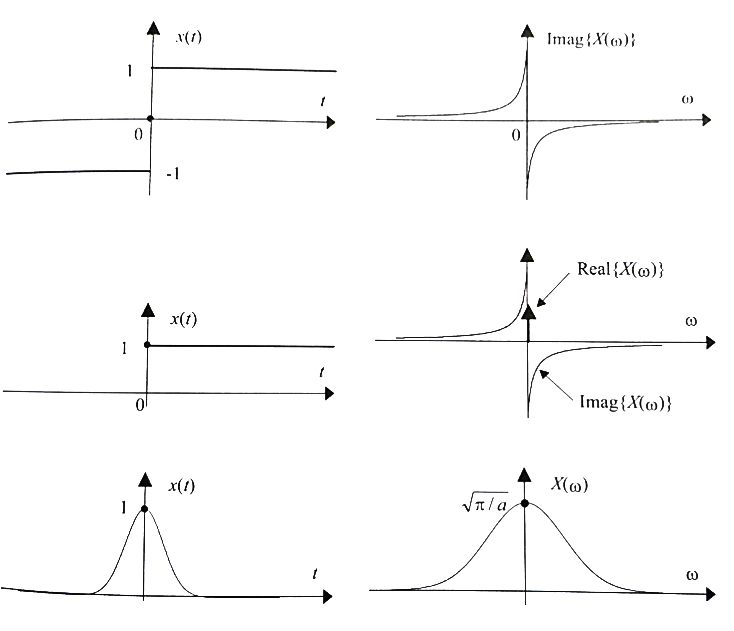
• for any real signal $f(t)$, Fourier transform has the following properties:
  • $\Re(F)$ - is an even function
  • $\Im(F)$ - is an odd function
  • $\lvert F \rvert$ - is an even function
  • $\angle(f)$ - is an odd function
• if $X$ isn't symmetric as above, FT isn't a real function (it's complex)
• additionally:
  • if $f(t)$ is real and even - $F(\omega)$ is also real and even
  • if $f(t)$ is real and odd - $F(\omega)$ is completely imaginary and odd
• since every singal can be decomposed into its even and odd part:
  • the even component of $f(t)$ corresponds to the $\Re[F(\omega)]$
  • the odd component of $f(t)$ corresponds to $i\Im[F(\omega)]$

Parseval theorem

\begin{equation} \int_{-\infty}^{\infty}f(x)g^{*}(x)\ dx=\int_{-\infty}^{\infty}F(\xi)G^{*}(\xi)\ d\xi \end{equation}

Plancherel theorem

\begin{equation} \int_{-\infty}^{\infty}||f(x)||^2\ dx=\int_{-\infty}^{\infty}||F(\xi)||^2\ d\xi \end{equation}

• Signal power:

\begin{equation} P=\lim_{T\rightarrow\infty} \int_{-\infty}^{\infty} |f(t)|^2 dt \end{equation}

• For discrete signals:

\begin{equation} \sum_{n=0}^{N-1}|x[n]|^2 = \frac{1}{N} \sum_{k=0}^{N-1}|X[k]|^2 \end{equation}

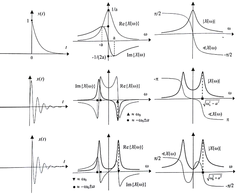
Examples